|
In this section we will learn about the graphs of power functions,
f(x) = ax p.
To examine these graphs, we will begin by considering a = 1 and p ≥ 0. Notice
that when
a = 1 all such power functions go through the point (1, 1) since,
f(1) = (1) p = 1.
Graphing power functions where x > 0 and p ≥ 0
In many biological applications, we are concerned with positive values of x, so
we will consider
f(x) = x p with x > 0 and p ≥ 0
by looking at several cases.
Case 1: p = 0
The graph of the function is a straight line, the constant function f(x) = 1.
Case 2: 0 < p < 1
The graph of the function is concave down and f(x) → ∞ as x → ∞.
Case 3: p = 1
If p = 1, the power function reduces to the linear function f(x) = x. This case separates the behavior of f(x) = xp for 0 < p < 1 and p > 1.
Case 4: p > 1
The graph of the function is concave up and f(x) → ∞ as x → ∞. |
One important feature of power functions is how they compare to one another
when
0 < x < 1 and x > 1. In particular, if 0 < x < 1, p > q implies xp < xq. For example, if 0 < x < 1,
then
x2 < √x. On the other hand, if x > 1, p > q implies xp > xq . For instance, if x > 1, then x2 > √x. This feature of power functions can be seen
in the plot below.

Graphing power functions where p ≥ 0 and x < 0
What happens to the function f(x) = x p when p ≥ 0 and x < 0 is more complicated.
\
- If p = r / s is a rational number expressed in lowest terms with s even or if p is an irrational number, f(x) = x p is not defined on the real line
when x < 0.
- If p = r / s is a rational number expressed in lowest terms with s odd, f(x) = x p is defined for negative values of x.
The graph of f(x) when x < 0 will
look one of two ways:
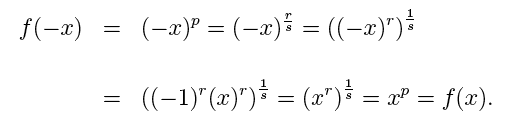
Case 1. If p = r / s (in lowest terms) with s odd and r even, f(x) → ∞ as x → − ∞,
and the graph of f(x) is symmetric about the y-axis (i.e. f(x) is even). To
see this, we interpret f(x) = xp as,

and we show f(x) is even (with r even) as,
The figure below depicts two such graphs.

Case 2. If p = r / s (in lowest terms) with s odd and r odd, f(x) → −1 as x → −1,
and the graph of f(x) is symmetric about the origin (i.e. f(x) is odd). To
see this, we interpret f(x) = x p as,

and we show f(x) is odd (with r odd) as,

The figure below depicts two such graphs.

Now we consider more complicated power functions where a ≠ 1 and p not necessarily
greater than zero. The case a ≠ 1 can be handled by recalling graphical
transformations. In particular, |a| > 1 vertically stretches the
graph with respect to the base graph y = xp, while |a| < 1 vertically shrinks the graph with respect to the base graph. If a < 0 there is also a reflection
about the x-axis.
Graphing power functions where p < 0.
The function f (x) = xp with p < 0 is not defined when x = 0 because division by zero is defined. Thus, we need to remove the point x = 0 from the domain since division by
zero is undefined. If negative values of x are in the domain of f(x) = xp (i.e. if
p = r / s in lowest terms with |s| odd), the behavior of f(x) near x = 0 increases or
decreases without bound. In particular, the line x = 0 is a vertical asymptote of
the graph. The graph of f(x) when p < 0 and f(x) defined for x < 0 will look
one of two ways:
Case 1. If p = r / s < 0 (in lowest terms) with |s| odd and |r| even, f(x) → ∞ as x → 0-
(i.e. as x approaches zero from the left), and f(x) → ∞ as x → 0 + (i.e. as
x approaches 0 from the right). The figure below depicts this behavior

Case 2. If p = r / s < 0 (in lowest terms) with |s| odd and |r| odd, f(x) → − ∞ as
x → 0- and f(x) → ∞ as x → 0+. The figure below depicts this behavior.

If negative real numbers are not in the domain of f (x) = xp with p < 0 (i.e. if p = r/s in lowest terms with |s| even or p is an irrational number), then f (x) → ∞ as x → 0+. The graph of f(x) will look lie the figure below.

*****
Now try some problems that will test your understanding of power functions.
Problems
|